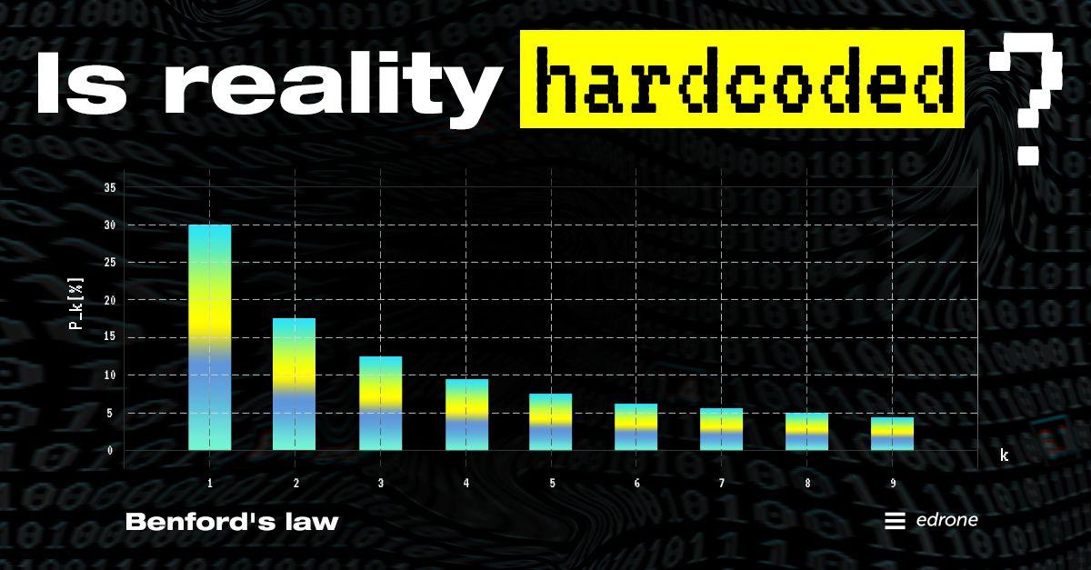
They aren’t random because they are determined by product prices! But what if I told you that there is a 33% chance that the cart value will start with the digit ‘1’?

Still not convinced? Take a look at the rest of the starting digits!

The data we took from the last few months

Hey, edrone, you have strange customers then! Once again, the answer is no. The eCommerce operations we work with are entirely “normal,” and it’s not a coincidence that the chart looks like this. It’s a universal phenomenon called Benford’s Law. It applies not only to eCommerce.

Before we dive into it and discuss what you can actually use this knowledge for (it is not only exciting curiosity!), let’s start from the basics to make sure we are on the same page.

Divination with some certainty

As an eCommerce manager, you have your trust in stats. You need them to inform decisions on actions you take every day. Still statistics aren’t always the rock-solid source of information you might think. Well, being honest, it is, but there is nothing wrong with that. The problem starts when somebody wants to treat stats deterministically, to get knowledge of what precisely will happen. That’s different than thinking that statistics will give you a clue about what will happen with some certainty.

Slice-and-dice

Take a look at a classic example – a standard 6-sided dice. For simplification, let’s call it ‘d6’. You have no clue which values out of six you will get when you roll the dice just once, but when you perform 600,000 throws, it’s more than certain that you will have around 100,000 of each value available on six-sided dice. It’s so because you know the probability distribution of the possible results; it’s even, which means each of them has the same chance to occur.

D6 dice are a good starting point because their values are entirely random. You cannot influence the result, or better to say, nothing affects it. Of course, you can cheat using doctored dice, but that’s not the case here, and also, such a die doesn’t give you significantly bigger chances to win a single roll.

Cart values are another cup of tea. Its values are chaotic, dependent on many factors, yet as you could see, somehow predefined. Cool things will start to happen when you begin to throw multiple dice, add the results, and count them down.

Feature of reality

With more factors, the effect is different from a simple linear probability distribution. The sum of dots varies from two to twelve, but in most cases, what you will get is a 7.

It can be easily explained when we will color the dice. ‘7’ has the biggest chance of being rolled as it can be reached thanks to two combinations of 1 & 6, two combinations of 2 & 5, and two combinations of 3 & 4. So the linear distribution starts to bend.

The more dice we add, the more it looks like a bell. Three dice:

And four dice.

The last example looks almost exactly like the star of our next section—normal distribution.

Insight One: With lots of samples, we can predict how aggregated results will look like.

Gauss curve, Normal Distribution

One of the most prominent aspects of the distribution is the Gaussian distribution. It’s backed with the central limit theorem.

The central limit theorem states that if you have a population with mean μ and standard deviation σ and take sufficiently large random samples from the population with replacement text annotation indicator, then the sample’s distribution will be approximately normally distributed.

In other words, when random, independent variables (e.g., d6 throws,) are added (the multiple throws shown above), their distribution converges to the normal distribution.

The last example was precisely this case—the sum of four randoms factors, with 1296 samples. Every single throw hadn’t normal distribution, and as a result of adding, we’ve ended with the normal distribution.

Let’s talk about real-life examples.

High School leaving exam

One of Poland’s most important school exams is a perfect example of how normal distribution works… and how beautifully it is apparent is that results are biased by those who check them.

The results should look like a regular bell curve. Occasionally it may move slightly to the right, due to better scores when the exam was easy, and to the left (lower scores) when it was tough.

In practice:

Two interesting things here. The first is that my result is somewhere there. The second is a gap around a score of 20 points. Based on the second clue, guess the pass threshold.

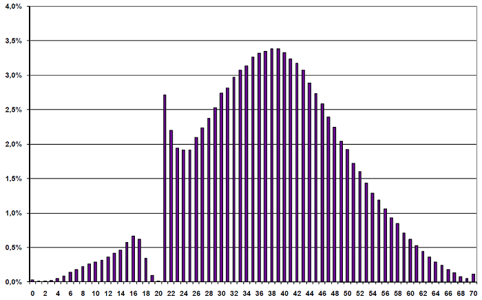
None of the teachers evaluating students’ work wants to fail any of them. Simply put, this exam is something essential, and if a test-taker sees that a student is literally a few points short of passing the exam, he or she is inclined to grade a few exercises more favorably.

Insight Two: With lots of samples, we can find out if somebody manipulated the data.

However, every student can, in theory, pass an exam with 100% correct answers. It is improbable, but what is essential is that each sample (student) is working independently. If he or she loses points, no one else is gaining them. On the other hand, earning points doesn’t require stealing them or taking them from the finite pool. E.g. money?

Pareto’s distribution

Gaussian decomposition applies in a sense to inanimate things. The Pareto principle seems to influence our decisions.

It is described by the Pareto decomposition and is also called the 80/20 rule. Its second name also describes its operation quite well.

• 20% of customers generate 80% of the revenue in your store
• 20% of employees in your store do 80% of all the “work”
• 20% of actions during eCommerce implementation make 80% of its effectiveness

And also more… hardcore

• 20% of the text conveys 80% of the information
• 80% of the mass of meteorites that have fallen to earth comes from 20% of the falls
• In the 20% biggest cities, lives 80% of humankind population.

Insight Three: With lots of samples and knowledge about the nature of phenomena, we can tell what type of distribution we are facing.

Benford’s Law in the new light

Finally, we’ve reached the law from which we started.

Let’s put together what we’ve learned so far.

• Insight One: With lots of samples, we can predict what aggregated results will look like.
• Insight Two: With lots of samples, we can find out if somebody manipulated the data.
• Insight Three: With lots of samples and knowledge about the nature of phenomena, we can tell what type of distribution we are facing.

I hope you now have a strong background to face Benford’s Law. Now let’s find out if reality is hardcoded.

Shall we, Mr Benford?

First and foremost, Benford’s law can be applied only for values that span over several orders of magnitude. So if values vary from 1 to 10, there is no chance to observe this effect. You will soon see why.

So what’s the explanation of this phenomena?

Lottery tickets are part of the best explanation I have seen.

Imagine that you are counting the probability of taking a number with ‘one’ at the beginning of the pool.

We start with one lottery ticket. Chance equals 100%; let’s write it down and start adding more tickets. With the number 2 in the pool, we lowered the chances to 50%. After adding the third, the probability drops to 1/3.

1 -> 1/1 = 1
2 -> 1/2 = 0.5
3 -> 1/3 = 0.3
[…]
9 -> 1/9 = 0.11

When we have nine tickets, chances for winning equals 1/9, but when we add the 10th ticket, it starts to rise:

10 -> 2/10 = 0.2
11 -> 3/11 = 0.27
12 -> 4/12 = 0.33
13 -> 5/13 = 0.38
[…]
19 -> 11/19 = 0.58

When we reach 20 tickets, chances once again start to drop until we get 100. In the range 100 – 199 tickets, the chances rise. Then start to fall in 200 – 999. And so on, and so on.

Distances between ups and downs are getting bigger and bigger since we are talking about continuous powers of 10. When we put it into a logarithmic scale, the chart will look, more or less, as a blade saw.

The logarithmic scale uses the next powers of ten instead of numbers as one step. Instead 1, 2, 3, 4; you have 1, 10, 100, 1000. We have to count the average value, and this value appears to be… 0,301.

To calculate the corresponding probabilities of left digits (same as 1), we can use the following equation.

[ {P(d)= log_{10} (1+1/d) } ]

d – digit we analyse

We get the following values.

1 -> 0.30103
2 -> 0.17609
3 -> 0.12494
4 -> 0.09691
5 -> 0.07918
6 -> 0.06695
7 -> 0.05799
8 -> 0.05115
9 -> 0.04576

But why is it exactly one?

Simply because counting towards something, you always start with 1. You have to count through ‘one’ when you are counting to 7. Trough 10 when counting to 40; 100 when 300. There is no certainty that your starting digit will be 1 at all. But if it’s for some reason the 9, there was a chance that it could have been the 1 because you went through it, counting whatever your number describes, which means it is included in your value range. If your value starts from 1, there is no such guarantee.

What can we use it for?

It is a feature of reality that can be easily observed while we look at multi-magnitude values. The perfect example is the population of cities worldwide. Note that these values also fit the Pareto distribution!

More or less, if values apply to Pareto’s distribution and span over several orders of magnitude, you can apply Benford’s Law to it. More precisely:

• When the median is lesser than the mean (distribution is down curved):

for {1, 6, 6, 6} set:
meen = 4,75
median = 6

for {1, 1, 1, 6} set:
meen = 2,25
median = 1

• When the skew is positive (right tail is longer then the left one)

So for what can we apply it to in practice? To lots of things!

• Accounting and finance, loan data
• Credit card transactions, customer balances, Stock prices
• National GDPs, populations of cities worldwide
• Purchase orders, inventory prices, transactions, customer refunds

But also:

• IT: computer file sizes
• Biology: protein lengths
• Physics: spectrum line intensity in complex atomic transition spectroscopy, hadron lifetime, the energy loss rate of pulsar self-rotation slowing, operation law of the objects outside the solar system in astronomy

Down-to-earth applications:

• Accounting and finance – the tax frauds detections
• Microeconomics – training the probability perception
• “The BL in the classroom” experiment.

I bet that from today you will be looking at digits differently 😉